A few months ago I was nerd sniped by a passing app idea
from an ex-colleague who coaches his son’s little league baseball team; “What if
we built an app that given a baseball teams batting stats, produced an optimal
lineup for that team”. Having grown up playing baseball and spending an almost
embarrassing amount of my childhood watching the movie The Sandlot, I was intrigued.
While I was still playing, I understood the conventional wisdom of put your highest
on base hitters in the 1, 2, and 3 slots, and your biggest slugger in the 4 slot. The general
idea is you want to load the bases for someone to hit big and bat those runners in,
and you want that pattern to appear as much as possible throughout the game, so it
has to be in the beginning of the lineup. But I never heard any theories on what
to do with the rest of the lineup, or seen actual statistic proof that this was
an optimal strategy.
Approaching the problem “How do you find an optimal lineup of players given their
batting statistics” is a bit of a daunting task. There are 2 major sub-problems
that need to be solved:
We need a way of comparing lineups and proving one is better than another. This allows
us to determine a sort order.
Once we have a way of comparing, a lineup of 9 players has 9! permutations; in other words
there are 362,880 different orders that you can put a lineup of 9 players. To find the
best one, there is a log of searching todo. Worse yet, little league can have longer linesups,
which grow factorially.
My initial naive approach was to write a simulator and randomly simulate baseball games
given each players likelihood of hitting and advancing the bases at any given
at bat. That went a little like:
from dataclasses import dataclass from enum import Enum, auto from itertools import cycle, permutations, repeat import random from typing importList, Tuple from statistics import mean from multiprocessing import Pool, cpu_count, freeze_support from multiprocessing.dummy import Pool as TPool import json from tqdm import tqdm
### Brute Force Optimization deflineup_expected_value(team: List[Player], iterations: int = 10000) -> float: with TPool(16) as pool: results = pool.map(simulate_team, repeat(team, iterations)) return mean(results)
defevaulate_lineup(lineup: List[Player]) -> Tuple[str, float]: lineup_name = "".join(player.name for player in lineup) expected_value = lineup_expected_value(lineup) # print(f"{lineup_name=} {expected_value=}") return lineup_name, expected_value
if __name__ == "__main__": total = sum(1for _ in permutations(team)) print(f"Brute Forcing {total} lineups") freeze_support()
with Pool(cpu_count()) as pool: lineup_values = dict(tqdm(pool.imap_unordered(evaulate_lineup, permutations(team)), total=total))
print(f'{lineup_values=}') print(sorted(lineup_values, key=lineup_values.get)) withopen('output.json', 'w') as output_file: json.dump(lineup_values, output_file)
Overall this approach uses the property of a statistical outcome that if you simulate
something enough times, you get a normal distribution centered around the weighted
average. Using some clever threading to speed up the simulation process, this
script attempted to simulate thousands of games and average the results to “score”
a lineup. This is a ok solution to problem #1, since we can now compare the scores
of any 2 given lineups, however this is subject to some error bars, since we are
taking an average of randomly generated results.
This also attempted to solve the second problem using threads, but being factorial
time, this was not fast. In an attempt to explore the space a bit more I booted some
heavy servers on AWS and ran this to get some results given some actual statistics from
a little league team provided my ex-colleague, but the time and cost of this compute
was a bit too high to justify.
So I put the problem down.
I will point out that after watching a bunch of Numberphile
and 3Blue1Brown videos
on youtube, I was aware of the Expected Value
calculation. I was particularly fascinated by a collaboration on the two channels
to find the expected value of a variation on a game of darts
that has a really elegant proof:
For those who dont nerd out over recreational maths, Expected Value is a way of calculating
the weighted average of a series of random outcomes without simulating them. It
is states as the sum of all of the values of all of the possible outcomes times
the probability of that particular outcome. So for baseball lineups, the expected
value would be the sum of all possible games and their scores times the chances that
any one given game was played given a lineup, totaled up.
So I knew this existed, but didn’t have enough of a grasp of how to go about calculating
it efficiently at the time. Paired with the other set of hard problems and the cost
of exploring the space, I was ready to close the book on it.
Fast forward to a few weeks ago, as I am studying more advanced dynamic programming
patterns, and using memoization to carve out repeated work in recursive trees; I
had a realization about the state of a baseball game and at bats. If any given at bat
has say 7 different outcomes on game state:
Strikeout (increase outs by 1, if new outs == 3, clear bases and advance inning)
Walk (Advance bases by 1, tallying new runs as they reach home)
Hit Out (Advance bases by 1 and increase outs by 1, following inning logic)
Single (Advance bases by 1)
Double (Advance bases by 2)
Triple (Advance bases by 3)
Homerun (Advance bases by 4)
Then the problem space for all possible games is 7n where n is the
number of at bats to playout an entire game. While n varys based on games, (a
game of all strikeouts only had 3 x num innings at bats, it is unlikely), it doesnt vary
enough to vastly change the search space.
My Realization is a game starting the second inning with no score and nobody on base
and the 5th batter coming to the plate has large number of ways it could get to
that game state. There could have been 1 hits and 3 strikeouts, 1 walk and 3 hit outs,
a mix of strike-outs and hits and hit-outs. What matters is not how the game go to
that state, but that the state of the game from that point to the end is the same
for the rest of the calculation, which means the entire subtree only needs to be
calculated once, or it can be memoized.
Taking a step back, one of the tenants of dynamic programming is memoization
of pure functions to reduce work. Take the following definition of fibonacci of n:
1
2
3
4
deffibonacci(n: int) -> int: if n <= 1: return n return fibonacci(n - 1) + fibonacci(n - 2)
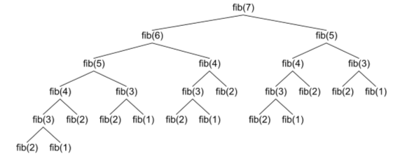
This very cleanly defines the nth fibonnaci number as the sum of the previous 2
fibonacci numbers. However its runtime is O(2n) since there is a ton of duplicated
work being done. To demonstrate, here is what the call tree for fibonacci(7) would look like:
Notice all of the duplicate calls. Memoization
allows us to store the results of a call in memory and return the result from memory
if that function is called with the same arguments again. This reduces the run time
from O(2n) to O(n) by trading a little bit of space. Python 3.9 has a helper
for memoization in functools called cached.
1
2
3
4
5
6
7
from functools import cached
@cached deffibonacci(n: int) -> int: if n <= 1: return n return fibonacci(n - 1) + fibonacci(n - 2)
To drive home how much of an improvement this is, if 1 call of fibonacci takes 1ms,
the un-memoized version of fibonacci(30) will take 12 days 10 hours 15 minutes to
complete, while the memoized version would take 30ms.
Back to baseball. Realizing that my search space of 7n for all possible games
could be drastically reduced using this same technique, I decided to give it a go
in python.
Using some other optimizations to reduce space and increase speed, I came up with:
@lru_cache(maxsize=None) defevaluate_lineup(players: Tuple[Player, ...], player_i: int = 0, game_state: GameRecord = None) -> float: if game_state isNone: game_state = GameRecord() if game_state.is_complete: return game_state.score returnsum( (probability * evaluate_lineup(players, (player_i + 1) % len(players), outcome_mapping[outcome](game_state)) for (outcome, probability) inzip(AtBatOutcome, players[player_i].outcome_chances) if probability) )
Key pieces to note, a GameRecord has to be hashable and to identical gamestates
need to hash to the same thing. This property comes nicely from dataclass(frozen=True)
which derives __hash__ and __eq__.
One caveat to expected value is since it is
exploring all of the possible games, there are games where nobody ever gets out. To
prevent this from causing an infinite loop, I used little league rules for a mercy
rule and capped the maximum runs in an inning to 5. Since all lineups will be measured
against this, this equally affects all lineups.
Here @lru_cache(maxsize=None) is the python 3.8 way of using functools.cached.
In python 3.9. cached is defined as lru_cache(maxsize=None).
Players here is cast to a tuple to make it hashable so it can be used as a key in
the memoization of the function. It is possible to pull this pieces out and memoize
just the index of the player (player_i) and the game state if you have closed
over the list of players, but that would mean the python runtime would have to
restart to clear the memoization table after each lineup was evaluated to
prevent it from always giving the same answer.
There is a lot of DRYing up that can be done with the game record management, however
this was very simple to write and during the actual runtime the changing of gamestate
will almost always be served out of the memoization cache.
Then the core of the evaluation is this piece:
1
2
3
4
5
6
7
8
9
10
def evaluate_lineup(players: Tuple[Player, ...], player_i: int = 0, game_state: GameRecord = None) -> float:
    if game_state is None:
        game_state = GameRecord()
    if game_state.is_complete:
        return game_state.score
    return sum(
        (probability * evaluate_lineup(players, (player_i + 1) % len(players), outcome_mapping[outcome](game_state))
         for (outcome, probability) in zip(AtBatOutcome, players[player_i].outcome_chances)
         if probability)
    )
Which comes directly from the expected value function. If a game state is completed
(it is has surpassed the max innings), it returns the score of the game. Otherwise
it returns the 7 possibilities an at-bat can produce times the recursive call
that has the new game state applied with the next player at bat.
In practice, a game that starts with 1 homerun and the rest of the entire game is strikeouts,
has a final score of 1. This contributes to the final expected value of the lineup
by:
So this score of 1 is multiplied by the very small probability that this was the game
that was played with this lineup. But then we sum that with the values of all of
the other games and their probabilities to get a definitive value.
So I took the same team that we have previously used in doing the simulations
and fed it into this algorithm, and in ~30 seconds, it returned a value. After
repeated runs, it returned the exact same value, partially showing that this
algorithm was deterministic (it should be since all of its parts are pure). After
swapping the order of 2 players, I got a different value; as expected.
So I had an algorithm for determining the expected value of a lineup and getting
a single value without error bars that are subject to randomness. This was exciting
as it in roughly the same amount of time as the simulation, but it gave a much
firmer answer. In theory running an infinite number of simulations should return
this exact answer.
This let me to the second problem, searching the factorial space of the different
permutations of lineups to find a maximum. At this point booting another clusters
of servers didn’t seem like the road I wanted to go down again. Another video
on youtube, this time from Computerphile
reminded me of a post on genetic algorithms I did a while back.
So given I have a function to evaluate a given order of a lineup, I can use that
as a fitness function to determine the survival of the fittest, and breed good
lineups together to produce (potentially) better ones. In theory, this algorithm
should quickly find local maximums then eventually get to a global maximum. One
of the points the video covers very well is the use of genetic algorithms to
explore a space and find out what the lay of the land of the space looks like.
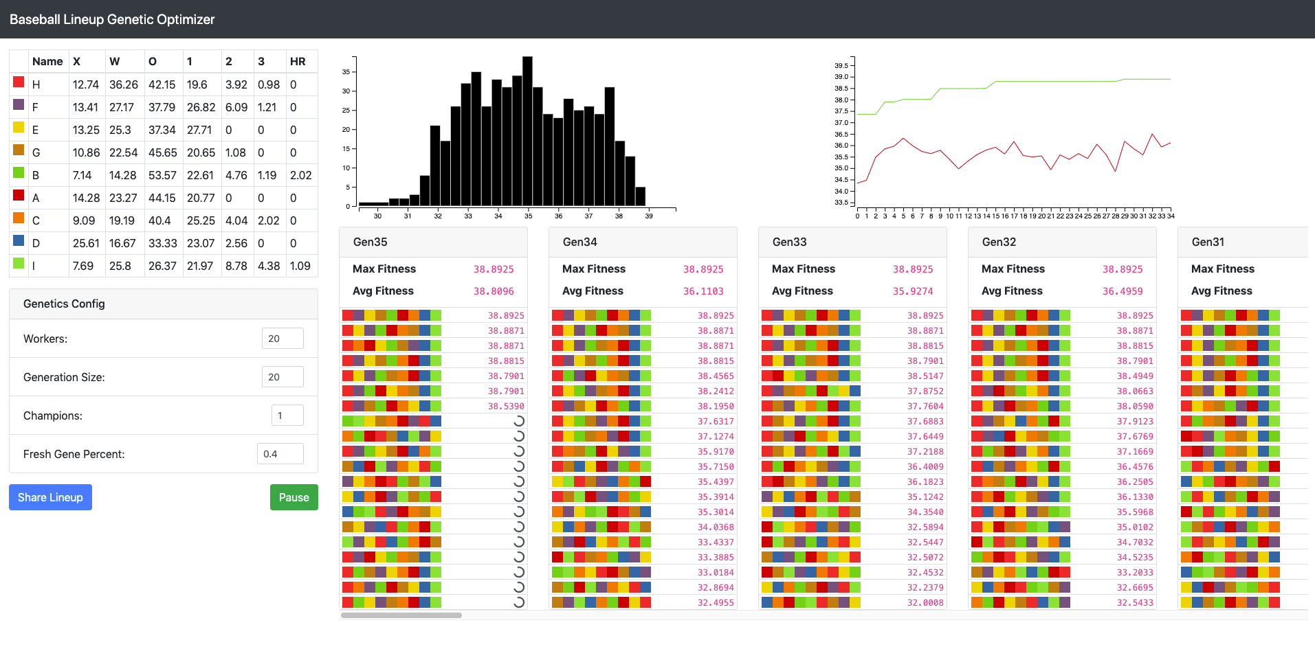
This game me an idea, to use the types of visualizations I used the last time I did a genetic algorithm to view species and trends. These visualizations could
show trends in the optimizations while the system was running. Doing all of this
visualization pushed me back to writing a web application. This expected value
function is almost the definition of a computationally heavy task, so I fell back
on the set of tools I used last time I needed to run a web application with computationally
heavy loads in parallel: WebAssembly paired with Web Workers.
The first step was rewriting the expected value function in rust:
Overall a bit more verbose since I dont have the same flexibility as I do with python,
but compiling it and running it in the browser was actually faster than the equivalent python.
I started down the path of writing my own javascript application to do the generation
of random lineups and the breeding of champions, however I quickly remembered how
much I hate doing state management and chasing weird edge cases in javascript, so
I wrote a Elm application to do all of the visualization and user interactivity.
To run with the exact data set I used, I added a share link that allows you to
quickly get started with the team loaded here
After watching it for a while, It does seem prioritize the traditional logic of
putting on-base hitters in 1,2,3 slots and a slugger in fourth, then putting some
minor copy of that pattern further down the lineup. Will be interesting to see
it run with different kinds of players to see what about those players have them
be more potent in those positions.
In retrospect I could also add a DIY lineup evaluator that allows you to try to
test your own theories while the genetic algorithm is running in the background
to see if you can intuitively beat the evolved algorithm, and if you can, have it
pull your intuition into the genepool to breed even better ones.
Overall it was a fun project dealing with cool computer science, cool web technologies
and cool visualizations to explore an interesting problem space.